Uniswap v3: The Universal AMM

Introduction

Uniswap v3 (paper) allows liquidity providers to provide custom amounts of liquidity in selected price ranges. This unlocks tremendous capital efficiency gains for liquidity providers who can manually adjust their exposure.

But this feature also greatly expands the design space for automated liquidity provision. Any static AMM can be approximated by a custom liquidity provision strategy involving multiple positions on Uniswap v3.

We can visualize the liquidity provided by any AMM as a curve in "tick space." Applying this method to existing AMMs like Curve, Balancer, and the logarithmic market scoring rule (LMSR) shows how those AMMs concentrate their liquidity across different prices, revealing the unique "liquidity fingerprint" corresponding to each of those AMMs.

Follow-up work will explore how strategies like this can be efficiently and accurately approximated in practice on Uniswap v3.

Automated market makers

This paper assumes you are familiar with automated market makers between two assets and that are defined as a trading function (see paper), meaning a relationship between its reserves and . We will only consider two-asset pools.

For ease of comparison, let's define the constants in each of these formulas in terms of , where is the quantity of when . You can loosely think of as the number of ``shares" that liquidity providers have in that pool. For example, the constant product formula used by Uniswap v2 (ignoring fees) can be described with the formula , with roughly corresponding to the total supply of liquidity tokens.

We will use to refer to the price of asset in terms of asset . is equivalent to the negated derivative of the reserves curve, . (For more background on thinking about AMMs in terms of derivatives, see the YieldSpace paper).

Uniswap v3

In Uniswap v3, anyone can create a position to provide some amount of liquidity——within a price range between two ticks. Tick indexes () are logarithmic in price, and specify the lower and upper prices at which that position provides liquidity.

As shown in the Uniswap v3 whitepaper, this is the trading function that describes the relationship between the reserves of a single Uniswap v3 position while its liquidity is in range:

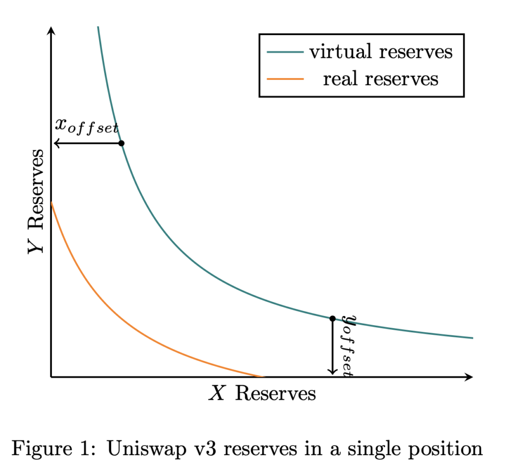
If a strategy involves providing liquidity in multiple positions, these definitions defined in terms of total reserves will no longer apply.

It would therefore be helpful to find a local definition for liquidity, that describes liquidity in its conventional sense: the pool's resistance to price impact when someone is trading with it.

As shown in Appendix A, it turns out that can also be defined as the rate of change of (the reserves of the token) for a given change in (the square root of the price of the token in terms of the token):

Simulating other curves

How can liquidity providers use Uniswap v3 to simulate a custom curve? One intuitive way to do so is to create many different positions, with a custom amount of liquidity in each:

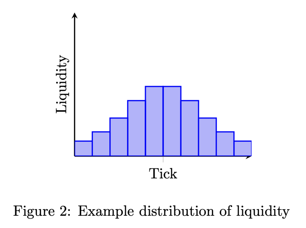
The more narrow these "slices" are, the more accurately this will simulate the target curve. For this post, we will treat tick space as infinitely divisible, and imagine that a liquidity provider is allowed to provide any arbitrary function to provide that amount of liquidity at any tick.

Graphing the function shows us the "liquidity fingerprint" of these other AMMs. (For convenience in defining functions of ticks, we will define as , as if our tick size was .) Appendix B shows the steps to derive this function from a given invariant.

Uniswap v2

The behavior of the reserves in Uniswap v2 can be described with the following equation:

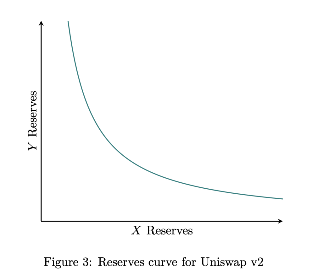
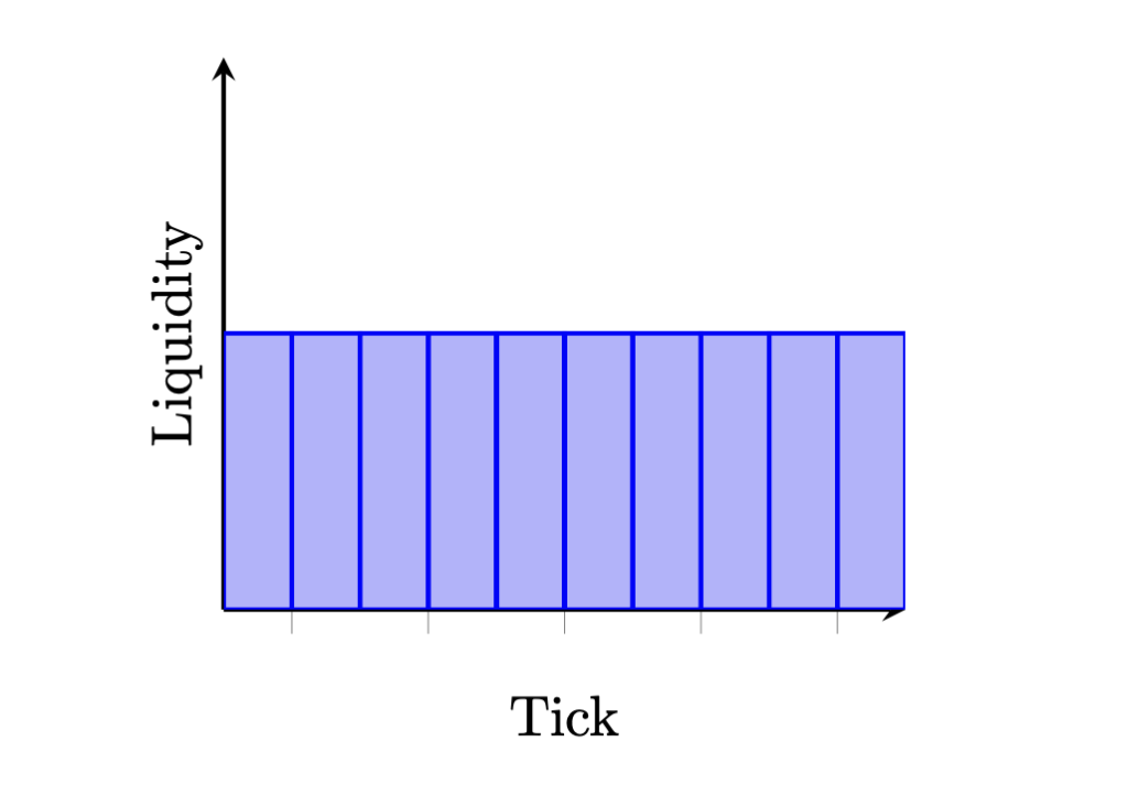
The liquidity fingerprint of this curve is a flat line:

To simulate this curve in Uniswap v3, we can simply create a single position with liquidity , and set our tick boundaries to and .

Curve (with constant chi)

The formula used by Curve is described in the StableSwap whitepaper. That paper first describes its invariant in terms of a constant amplification factor, . Their formula can be written as:

This reserves curve (with Uniswap v2 shown for comparison) looks like:

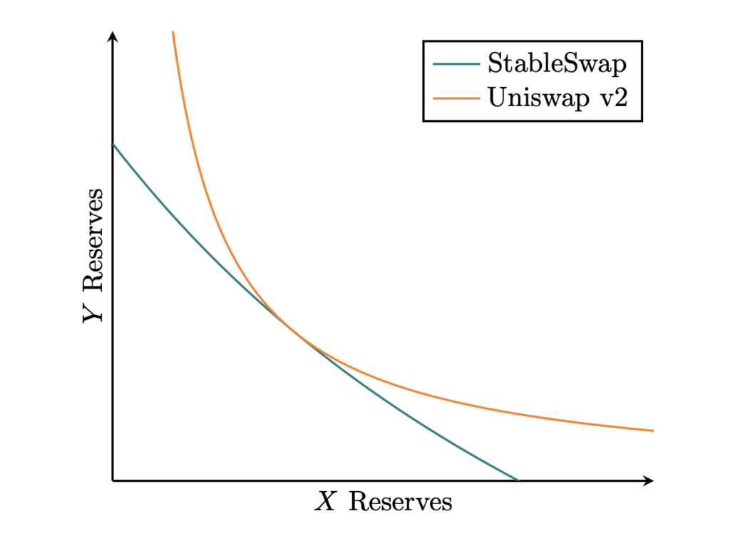
It turns out that with a constant , the liquidity provided by this formula is exactly equivalent to a single Uniswap v3 position, if we set ), and set the upper and lower prices to and . This means that we can simulate this formula with a single position in Uniswap v3:

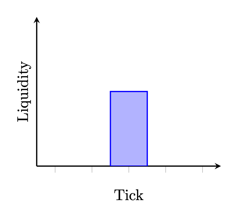
Curve in fact uses a non-constant , which is defined (using our terminology) as , where A is a constant amplification factor. This leads to a more complicated equation that is harder to represent with a closed-form liquidity function. In follow-up work, I'll show how to approximate this and other curves numerically.

Balancer

The reserves in a two-asset Balancer pool can be described by this invariant, where is the weight of the asset and is the weight of the asset (or ):

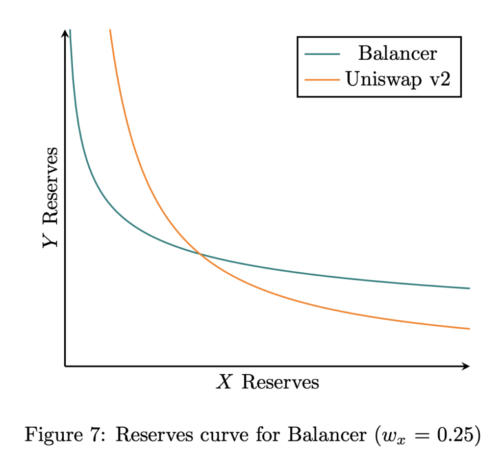
In liquidity space, this corresponds to an exponential function:

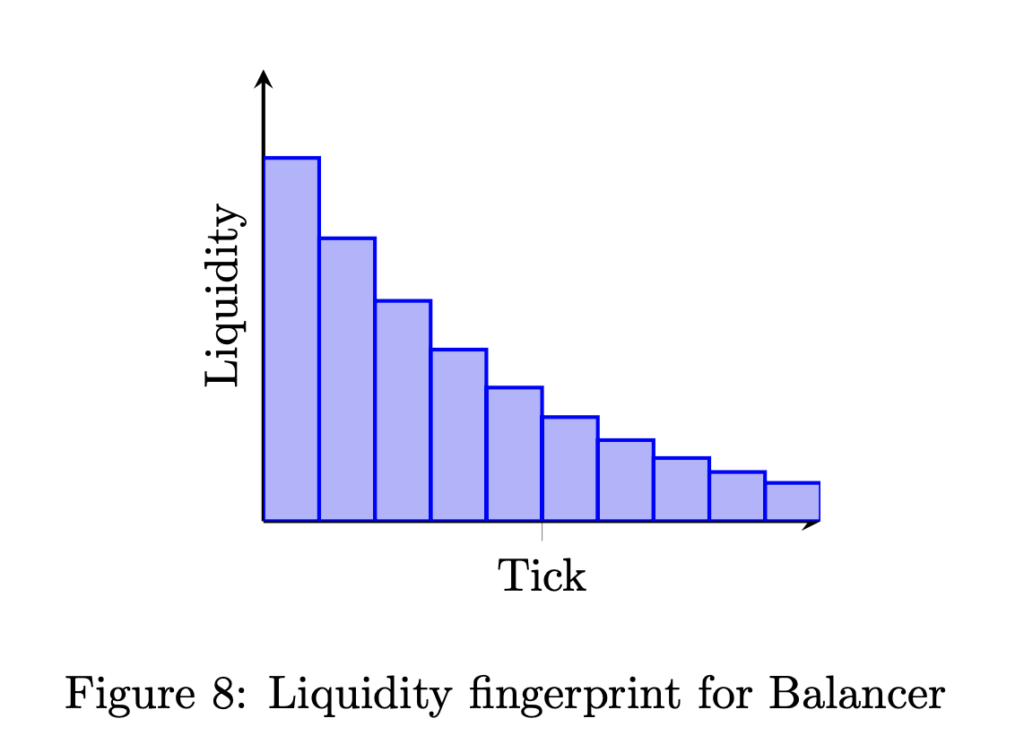
Intuitively, when asset is weighted less heavily, more of the pool's liquidity is reserved for lower prices of asset . This makes sense, because at any given time, liquidity reserved for lower prices is effectively buy orders for asset , so it is currently held in asset .

Logarithmic market scoring rule

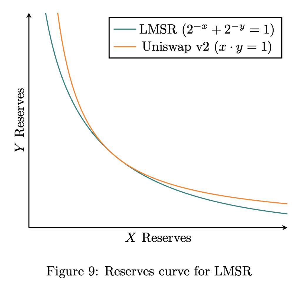
The logarithmic market scoring rule (LMSR) is one of the first and most widely studied automated market makers. The two-asset case is best known for its application to a binary prediction market (i.e., between YES and NO shares), where the price of the two assets (in cash) adds up to 1.

Typically, LMSR is described in terms of the rule for market-making between each asset (YES and NO) and cash. We could instead describe it in terms of the rule for market-making between one asset and the other. If we do that, then as explained here, the reserves can be described by this invariant:

The reserves curve for this formula looks like:

When transformed into tick space, the liquidity fingerprint of this curve is shaped like—you guessed it—the hyperbolic secant function:

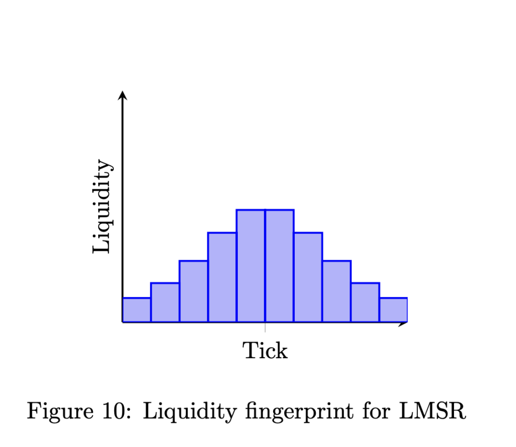
As you can see, LMSR concentrates more of its liquidity closer to tick 0 (the price of 1). In prediction markets, when YES and NO shares are equal, that implies a probability of 50%. So LMSR concentrates more liquidity to support probabilities around 50% than to support more extreme probabilities.

Appendix B shows how this liquidity fingerprint can be computed.

Future work

This paper showed how several popular AMMs could be simulated using Uniswap v3, and showed how graphing curves in liquidity space provides insight into their unique ``liquidity fingerprints". However, there are several limitations that need to be overcome before Uniswap v3 can be used to simulate most of these AMMs:

• Ticks are not infinitely divisible, and liquidity providers have to approximate this curve using the granular ticks available.
• The gas cost of minting and burning is proportional to the number of ticks updated, so providing liquidity at custom levels across all of tick space would be insurmountably inefficient.
• Finally, not every useful AMM can be easily represented as a function in liquidity space.

Future work will demonstrate some techniques for getting around these problems using numerical approximation, as well as some smart contract tricks to make custom liquidity provision much more gas-efficient.

Appendices

Appendix A: Definition of liquidity

We can show that in Uniswap v3, the derivative is equal to .

We start with the trading function (while the position is in range):

Solving for (to use later):

Solving for :

Finding as a function of by taking :

Solving for instead:

Substituting for and simplifying:

Solving for :

Taking the derivative:

Appendix B: Example derivation

This appendix shows how to go from an AMM formula defined as a trading function to a liquidity curve in tick space. We'll use LMSR as an example.

As shown in Appendix A, liquidity can be defined as the rate of change of with respect to . Since is simply -1 times the derivative of with respect to , we know that liquidity can be computed as:

We start with the AMM defined as an invariant:

Solving for :

Taking the derivative and negating it to get the price (of asset in terms of asset ) as a function of :

We then need to find the formula for that same price, but as a function of rather than . Since this curve (like the others described in this post) is symmetrical between and , we can easily get the price as a function of by replacing with and taking the reciprocal:

Next, we invert this to find as a function of , and then rewrite it as a function of .

Then we take the derivative with respect to :

Finally, we convert to tick space by rewriting this as a function of tick index ():